
Keyword Match vs. Semantic Relevance: How to Tell Whether a Ranking Is Good
Two ways to decide that a result fits a query, and a simple method for judging which ranking is better: measure it against people's judgments.
Synthetic dataExamples on this page use synthetic data created for illustration.
On this page
Search and recommendation systems have to answer two different questions. First: how do we decide that an item fits a query? Second, and harder: once we have a ranking, how do we know it is any good?
Two ways to say “relevant”
Keyword matching looks for the query’s words in the item. Better versions weigh the words: a word that appears often in this item but rarely elsewhere counts for more. BM25 is the best-known formula of this kind. It is fast, and you can always point at the words that caused a match. Its weakness is vocabulary mismatch: a search for “car” will miss a page that only says “automobile”.
Semantic matching turns texts into vectors of numbers so that similar meaning gives nearby vectors. It handles paraphrase and related concepts well. Its weaknesses are the mirror image: it can drift to things that are merely on the same topic, it often blurs negation, exact names and numbers, and it is harder to explain why an item matched.
Neither is simply better. Real systems often combine them. What decides between them is not argument but measurement.
Measure against judgments
The standard method is plain:
- Collect realistic queries.
- For each, have people grade the returned items, for example from 0 (not relevant) to 3 (exactly what was wanted).
- Compute a number for each approach and compare.
Counting how many good items are returned is a start. Precision and Recall do this. But two rankings can return the same good items and still differ a lot, because users read from the top. A good metric should reward putting the best items first.
A worked example
The grades below are synthetic. Two rankings return the same five items for one query, in different orders. The grades are listed by position.
| Position | 1 | 2 | 3 | 4 | 5 |
|---|---|---|---|---|---|
| Ranking A | 3 | 2 | 0 | 1 | 0 |
| Ranking B | 0 | 3 | 2 | 0 | 1 |
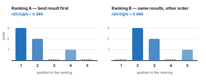
Both rankings have two relevant items in the top three, so precision at 3 is 2/3 for each. They are clearly not equally good: A puts the best item first.
Discounted cumulative gain (DCG) adds up the grades but discounts lower positions:
Dividing by the best possible DCG for the same items gives normalized DCG (nDCG), a score between 0 and 1.
| DCG@5 | Ideal DCG@5 | nDCG@5 | |
|---|---|---|---|
| Ranking A | 4.69 | 4.76 | 0.985 |
| Ranking B | 3.28 | 4.76 | 0.689 |
The ideal ordering for these items is grades 3, 2, 1, 0, 0. Ranking A is almost ideal; B is far from it. Precision could not see the difference. nDCG does.
Pitfalls
- Too few judged queries. Ten queries can mislead. Aim for dozens, and look at the spread, not only the average.
- Judges disagree. Write down what each grade means, and check how often two people give the same grade.
- Clicks are not judgments. People click what is shown first. Click data mostly measures position.
- Tuning on the test set. If you adjust the system until the judged set looks good, the score stops meaning anything. Keep some queries aside; this is Overfitting by another route.
- Not measuring after a change. A rule tweak that helps one query often hurts another. Re-run the same set every time.
A routine that works
- Write 30 to 50 realistic queries.
- Judge the top results for each, with a short written guide.
- Score each approach with precision, recall and nDCG.
- Read the worst failures by hand. They tell you more than the averages.
- Keep the judged set, and re-run it after every change.
Combining the two
Many production systems do not choose. They retrieve candidates with both methods, merge the lists, and let a ranking step decide the order. A simple way to merge is reciprocal rank fusion: each list gives an item 1 / (60 + position) points, and the points are added. An item that is near the top of both lists beats an item at the very top of only one. Because the merge is arithmetic on positions, it needs no tuning of scores that live on different scales, and every point can be explained (“it was third in the keyword list and second in the meaning list”).
Whichever way the two are combined, the same judged queries decide whether it helped. Run the keyword method alone, the meaning method alone, and the combination over the same judged set, and compare their nDCG. If the combination does not beat the better of the two, it is adding complexity without adding quality.
In short
Keyword matching is transparent and brittle; semantic matching is flexible and opaque. Which one fits your case is an empirical question, and the only reliable answer is a small, honest, repeatable measurement.
References
- Christopher D. Manning, Prabhakar Raghavan, Hinrich Schütze. Introduction to Information Retrieval . Cambridge University Press, 2008. ISBN 978-0521865715.
- Kalervo Järvelin, Jaana Kekäläinen. Cumulated Gain-Based Evaluation of IR Techniques . ACM Transactions on Information Systems, 2002. DOI: 10.1145/582415.582418
- Stephen Robertson, Hugo Zaragoza. The Probabilistic Relevance Framework: BM25 and Beyond . Foundations and Trends in Information Retrieval, 2009. DOI: 10.1561/1500000019
- Gordon V. Cormack, Charles L. A. Clarke, Stefan Buettcher. Reciprocal Rank Fusion Outperforms Condorcet and Individual Rank Learning Methods . Proceedings of the 32nd International ACM SIGIR Conference, 2009. DOI: 10.1145/1571941.1572114